How to use larda

Initialize

#!/usr/bin/python3
import sys
sys.path.append('<path to local larda directory>')
import pyLARDA
import pyLARDA.helpers as h

# optionally configure the logging
# StreamHandler will print to console
import logging
log = logging.getLogger('pyLARDA')
log.setLevel(logging.DEBUG)
log.addHandler(logging.StreamHandler())

# init larda
# either using local data
larda=pyLARDA.LARDA()
# or loading data via http from backend
larda = pyLARDA.LARDA('remote', uri='<url to larda remote backend>')
print("available campaigns ", larda.campaign_list)

# select a campaign
larda.connect('lacros_dacapo')

Load data

Get the data container for a certain system and parameter.

improt datetime
# Initialize larda as described above

begin_dt = datetime.datetime(2018, 12, 18, 6, 0)
end_dt = datetime.datetime(2018, 12, 18, 11, 0)

MIRA_Zg = larda.read("MIRA", "Zg", [begin_dt, end_dt], [0, 'max'])
#
shaun_vel=larda.read("SHAUN", "VEL", [begin_dt, end_dt], [0, 'max'])

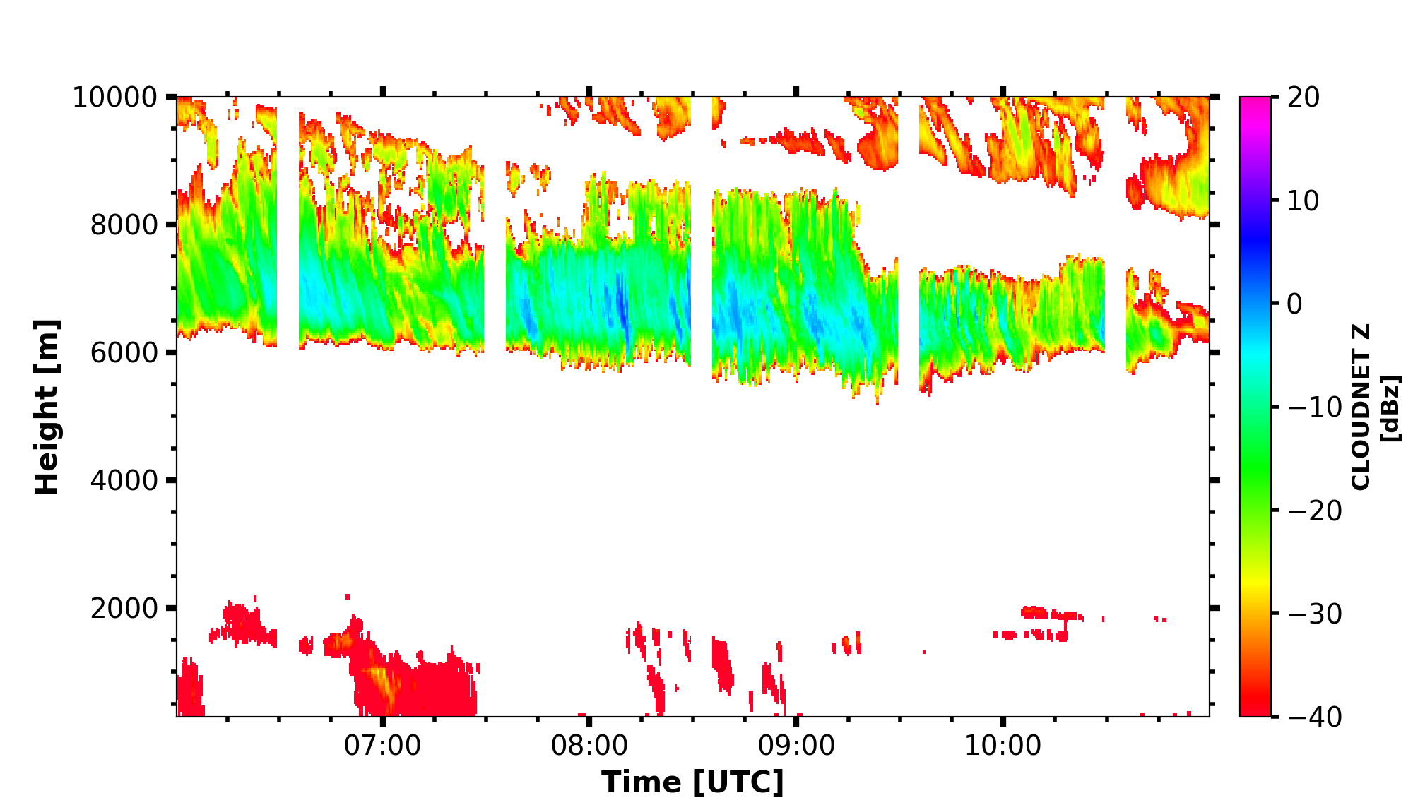
Simple plot

begin_dt = datetime.datetime(2018, 12, 18, 6, 0)
end_dt = datetime.datetime(2018, 12, 18, 11, 0)
CLOUDNET_Z = larda.read("CLOUDNET", "Z", [begin_dt, end_dt], [0, 'max'])
fig, ax = pyLARDA.Transformations.plot_timeheight(
    CLOUDNET_Z, range_interval=[300, 12000], z_converter='lin2z')
fig.savefig('cloudnet_Z.png')

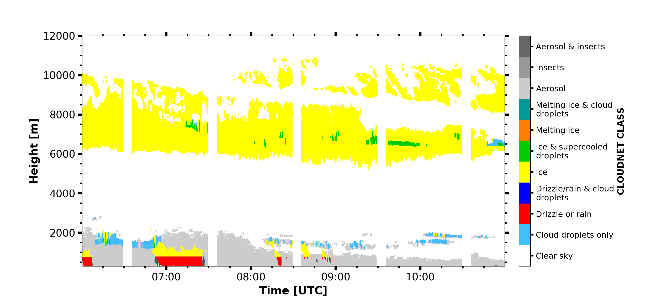
CLOUDNET_class = larda.read("CLOUDNET", "CLASS", [begin_dt, end_dt], [0, 'max'])
fig, ax = pyLARDA.Transformations.plot_timeheight(
    CLOUDNET_class, range_interval=[300, 12000])
fig.savefig('cloudnet_class.png')

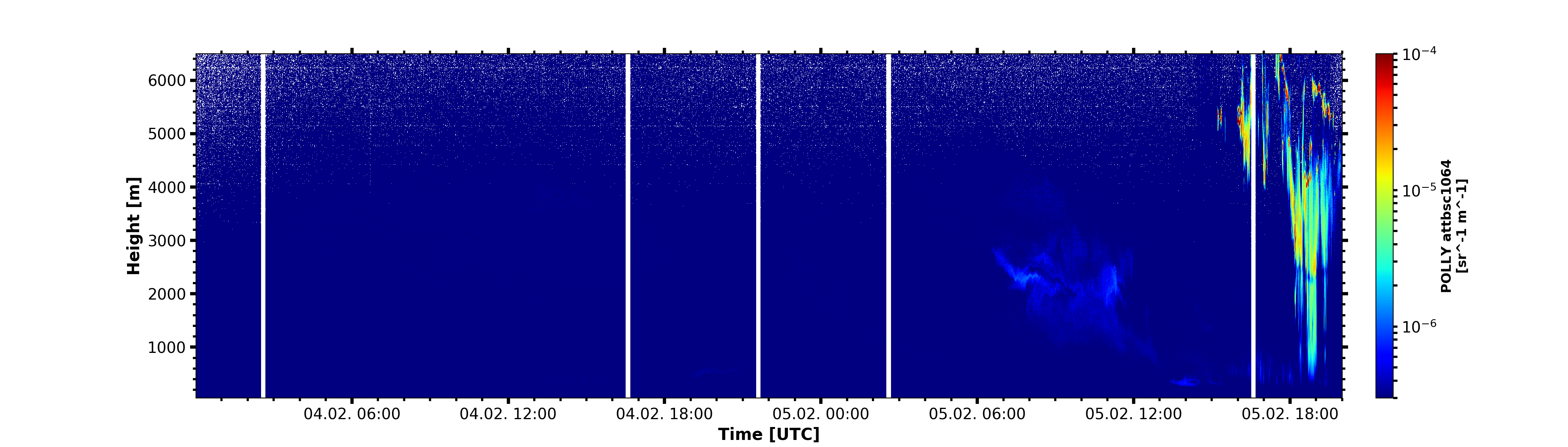
Modify plot appareance

begin_dt=datetime.datetime(2019,2,4,0,1)
end_dt=datetime.datetime(2019,2,5,20)
plot_range = [50, 6500]

attbsc1064 = larda.read("POLLY","attbsc1064",[begin_dt,end_dt],[0,8000])
attbsc1064['colormap'] = 'jet'
fig, ax = pyLARDA.Transformations.plot_timeheight(
        attbsc1064, range_interval=plot_range, fig_size=[20,5.7], z_converter="log")
ax.xaxis.set_major_formatter(matplotlib.dates.DateFormatter('%d.%m. %H:%M'))
ax.xaxis.set_major_locator(matplotlib.dates.HourLocator(byhour=[0, 6, 12, 18]))
ax.xaxis.set_minor_locator(matplotlib.dates.MinuteLocator(byminute=[0,]))
fig.savefig('polly_bsc1064.png')

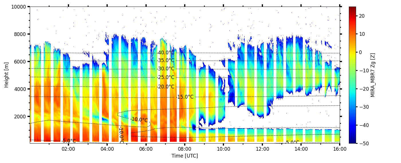
Overlay plot

larda.connect('cloudlab_III')

begin_dt=datetime.datetime(2024,1,8,0,0)
begin_dt2=datetime.datetime(2024,1,7,23,0)
end_dt=datetime.datetime(2024,1,8,16,0)
plot_range = [50, 10000]

T = larda.read("CLOUDNET","T", [begin_dt2,end_dt], plot_range)
def toC(datalist):
        return datalist[0]['var']-273.15, datalist[0]['mask']
contour = {
        'data': pyLARDA.Transformations.combine(toC, [T], {'var_unit': "C"}),
        'levels': np.arange(-40,11,5)
    }

MIRA_Zg = larda.read("MIRA_MBR7","Zg",[begin_dt,end_dt],[0,'max'])
MIRA_Zg['colormap'] = 'jet'
fig, ax = pyLARDA.Transformations.plot_timeheight2(MIRA_Zg, range_interval=plot_range, fig_size=[20,5.7], z_converter="lin2z",contour=contour)
ax.xaxis.set_major_formatter(matplotlib.dates.DateFormatter('%H:%M'))
ax.xaxis.set_major_locator(matplotlib.dates.HourLocator(byhour=[0,2,4,6,8,10,12,14,16]))
ax.xaxis.set_minor_locator(matplotlib.dates.MinuteLocator(byminute=[0,]))
fig.savefig('MIRA_Z.png')

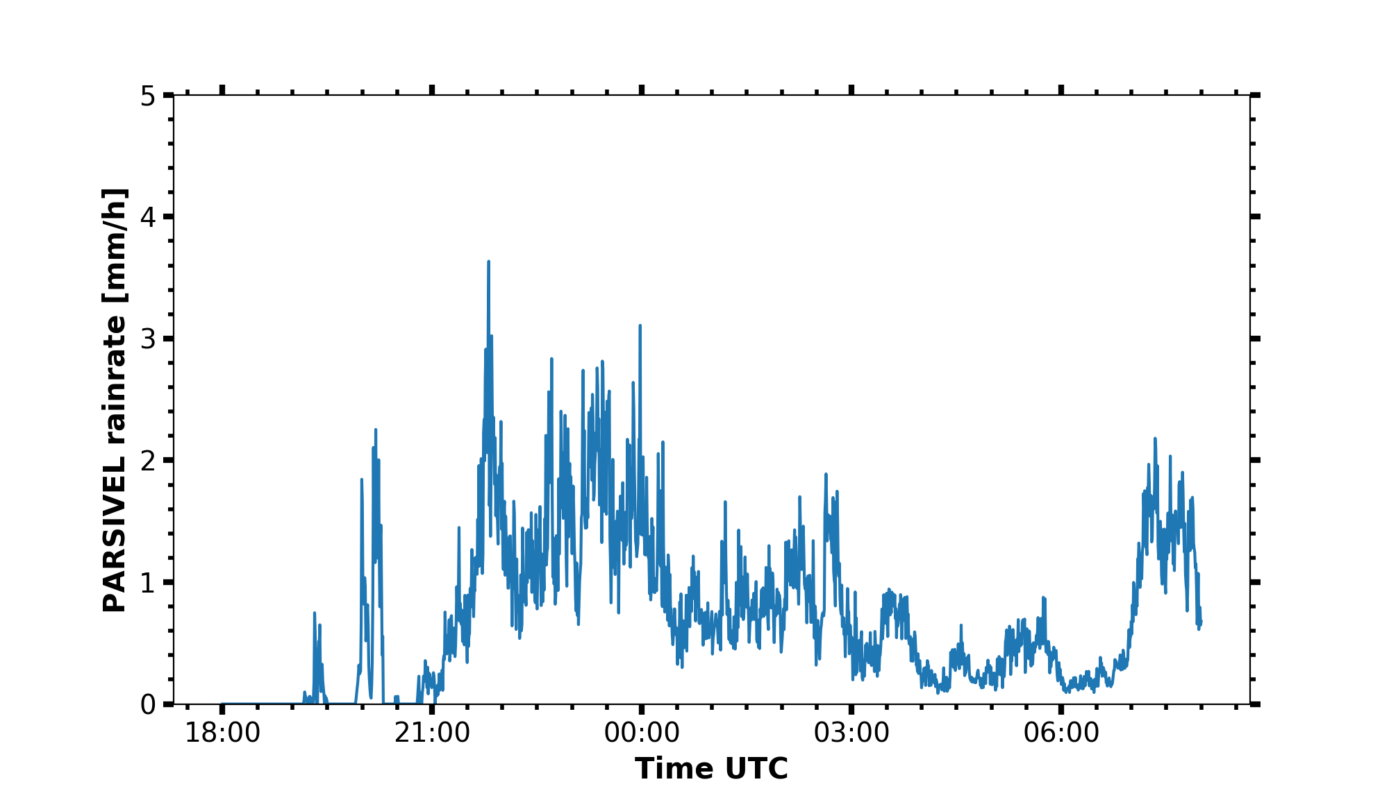
Timeseries plot

begin_dt = datetime.datetime(2019, 4, 8, 18, 0)
end_dt = datetime.datetime(2019, 4, 9, 8, 0)
parsivel_rainrate = larda.read("PARSIVEL", "rainrate", [begin_dt, end_dt])

#convert rainrate in m s-1 to mm h-1
# modify dict by hand
#parsivel_rainrate['var'] = parsivel_rainrate['var']*3600/1e-3
#parsivel_rainrate["var_unit"] = 'mm/h'
#parsivel_rainrate['var_lims'] = [0,10]

# or use the Transformations.combine syntax
def to_mm_h(datalist):
    return datalist[0]['var']*3600/1e-3, datalist[0]['mask']
parsivel_rainrate = pyLARDA.Transformations.combine(
    to_mm_h, [parsivel_rainrate], {'var_unit': 'mm/h', 'var_lims': [0,5]})
fig, ax = pyLARDA.Transformations.plot_timeseries(parsivel_rainrate)
fig.savefig('parsivel_rain_rate.png')

#to add more lines simply add them to the subplot
mrr_rainrate = larda.read("MRR-PRO", "rainrate", [begin_dt, end_dt])
#convert unix time to standard datetime format
time_list= [h.ts_to_dt(ts) for ts in mrr_rainrate['ts']]
ax.plot(time_list, mrr_rainrate['var'], label='MRR rain rate')
fig.savefig('parsivel_mrr_rain_rate.png')

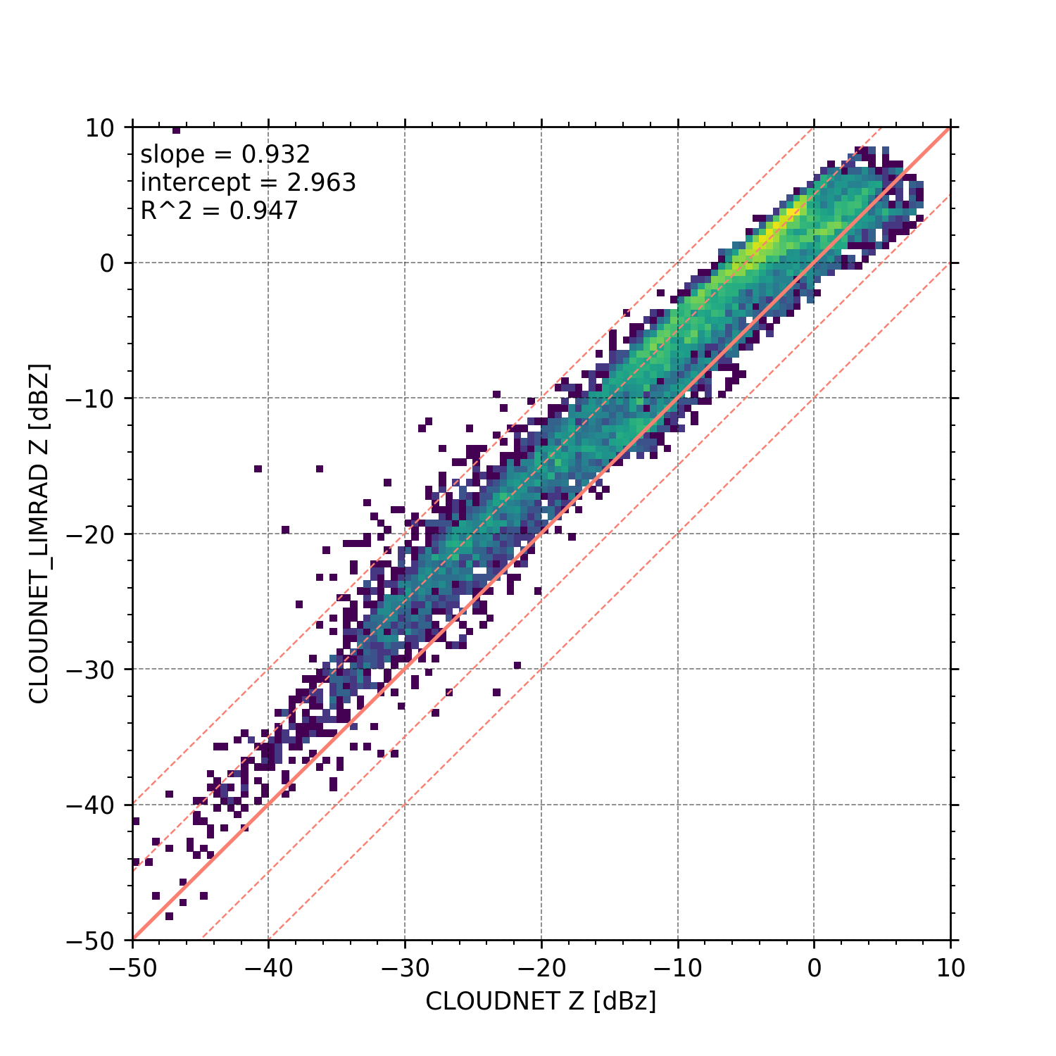
Scatter plot

begin_dt = datetime.datetime(2018, 12, 6, 0, 0, 0)
end_dt   = datetime.datetime(2018, 12, 6, 0, 30, 0)

# load the reflectivity data
MIRA_Z = larda.read("CLOUDNET", "Z", [begin_dt, end_dt], [0, 'max'])
LIMRAD94_Z = larda.read("CLOUDNET_LIMRAD", "Z", [begin_dt, end_dt], [0, 'max'])

LIMRAD94_Z_interp = pyLARDA.Transformations.interpolate2d(LIMRAD94_Z,
                                        new_time=MIRA_Z['ts'], new_range=MIRA_Z['rg'])
fig, ax = pyLARDA.Transformations.plot_scatter(MIRA_Z, LIMRAD94_Z_interp, var_lim=[-75, 20],
                                        x_lim = [-50, 10], y_lim = [-50, 10],
                                        custom_offset_lines=5.0, z_converter='lin2z')
fig.savefig('scatter_mira_limrad_Z.png', dpi=250)

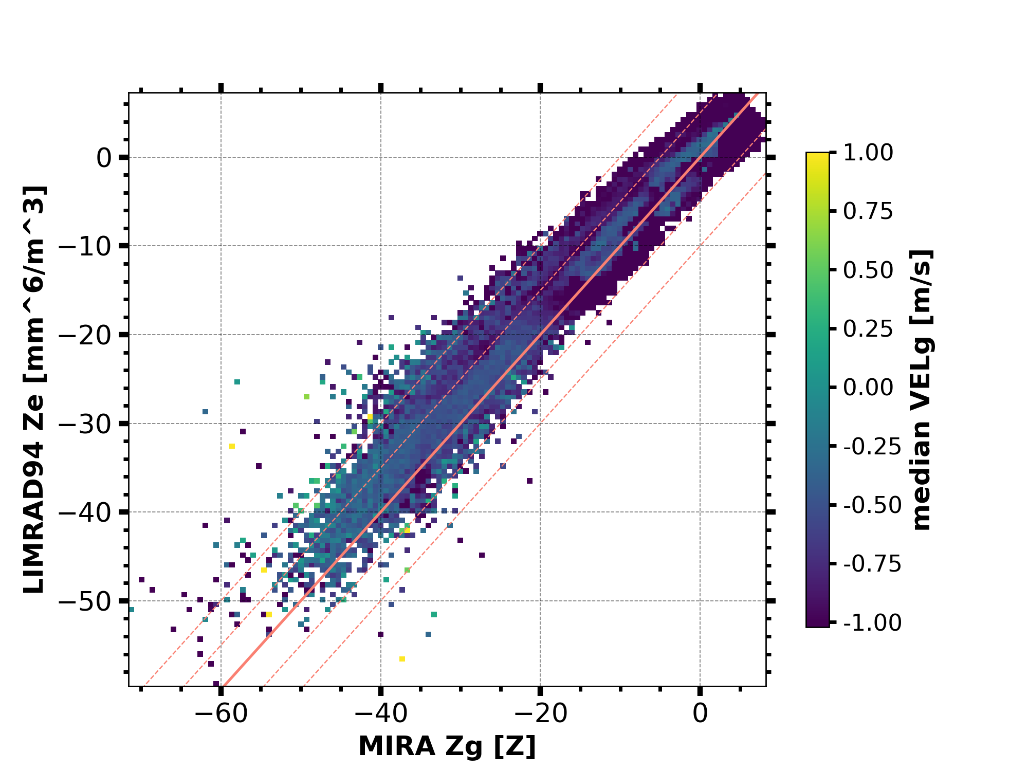
Scatter plot colored by additional variable

begin_dt = datetime.datetime(2018, 12, 6, 0, 0, 0)
end_dt   = datetime.datetime(2018, 12, 6, 0, 30, 0)

plot_range = [0, 12000]

# load the reflectivity data
MIRA_Zg = larda.read("MIRA", "Zg", [begin_dt, end_dt], [0, 'max'])
MIRA_Zg['var_lims'] = [-60, 20]

LIMRAD94_Z = larda.read("LIMRAD94", "Ze", [begin_dt, end_dt], [0, 'max'])
LIMRAD94_Z['var_lims'] = [-60, 20]

LIMRAD94_Z_interp = pyLARDA.Transformations.interpolate2d(
    LIMRAD94_Z, new_time=MIRA_Zg['ts'], new_range=MIRA_Zg['rg'])

# load the Doppler velocity data
MIRA_VELg = larda.read("MIRA", "VELg", [begin_dt, end_dt], [0, 'max'])
LIMRAD94_VEL = larda.read("LIMRAD94", "VEL", [begin_dt, end_dt], [0, 'max'])

fig, ax = pyLARDA.Transformations.plot_scatter(
    MIRA_Zg, LIMRAD94_Z_interp, var_lim=[-75, 20], z_converter='lin2z',
    custom_offset_lines=5.0, color_by=MIRA_VELg, scale='lin',
    c_lim=[-1, 1], colorbar=True)
fig.savefig('scatter_mira_limrad_Z_by_VEL.png', dpi=250)

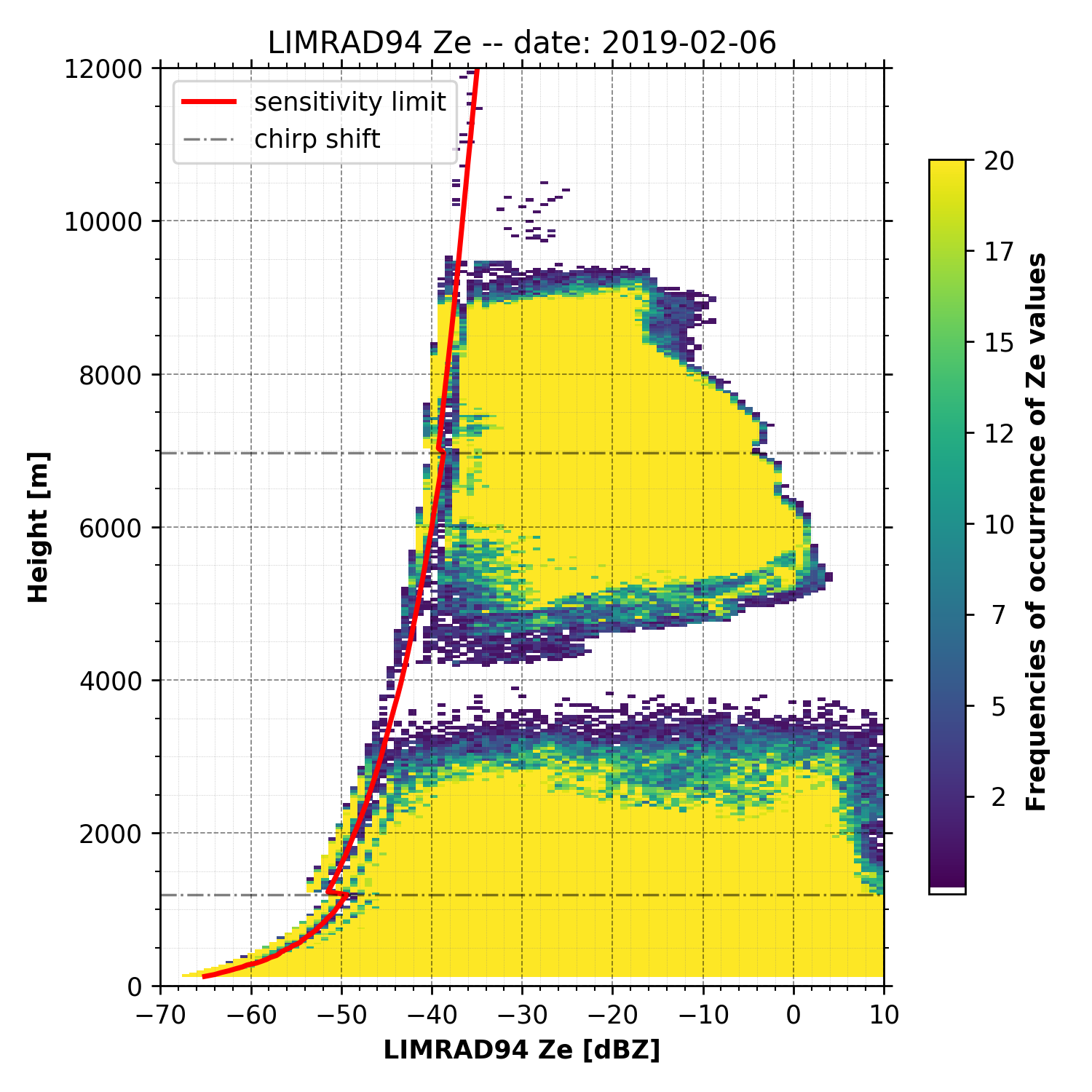
Frequency of occurence

begin_dt = datetime.datetime(2019, 2, 6)
end_dt = datetime.datetime(2019, 2, 6, 23, 59, 59)
plot_range = [0, 12000]

LIMRAD94_Ze = larda.read("LIMRAD94", "Ze", [begin_dt, end_dt], plot_range)
# load range_offsets, dashed lines where chirp shifts
range_C1 = larda.read("LIMRAD94", "C1Range", [begin_dt, end_dt], plot_range)['var'].max()
range_C2 = larda.read("LIMRAD94", "C2Range", [begin_dt, end_dt], plot_range)['var'].max()
# load sensitivity limits (time, height) and calculate the mean over time
LIMRAD94_SLv = larda.read("LIMRAD94", "SLv", [begin_dt, end_dt], plot_range)
sens_lim = np.mean(LIMRAD94_SLv['var'], axis=0)

fig, ax = pyLARDA.Transformations.plot_frequency_of_occurrence(
    LIMRAD94_Ze, x_lim=[-70, 10], y_lim=plot_range,
    sensitivity_limit=sens_lim, z_converter='lin2z',
    range_offset=[range_C1, range_C2],
    title='LIMRAD94 Ze -- date: {}'.format(begin_dt.strftime("%Y-%m-%d")))

fig.savefig('limrad_FOC_example.png', dpi=250)

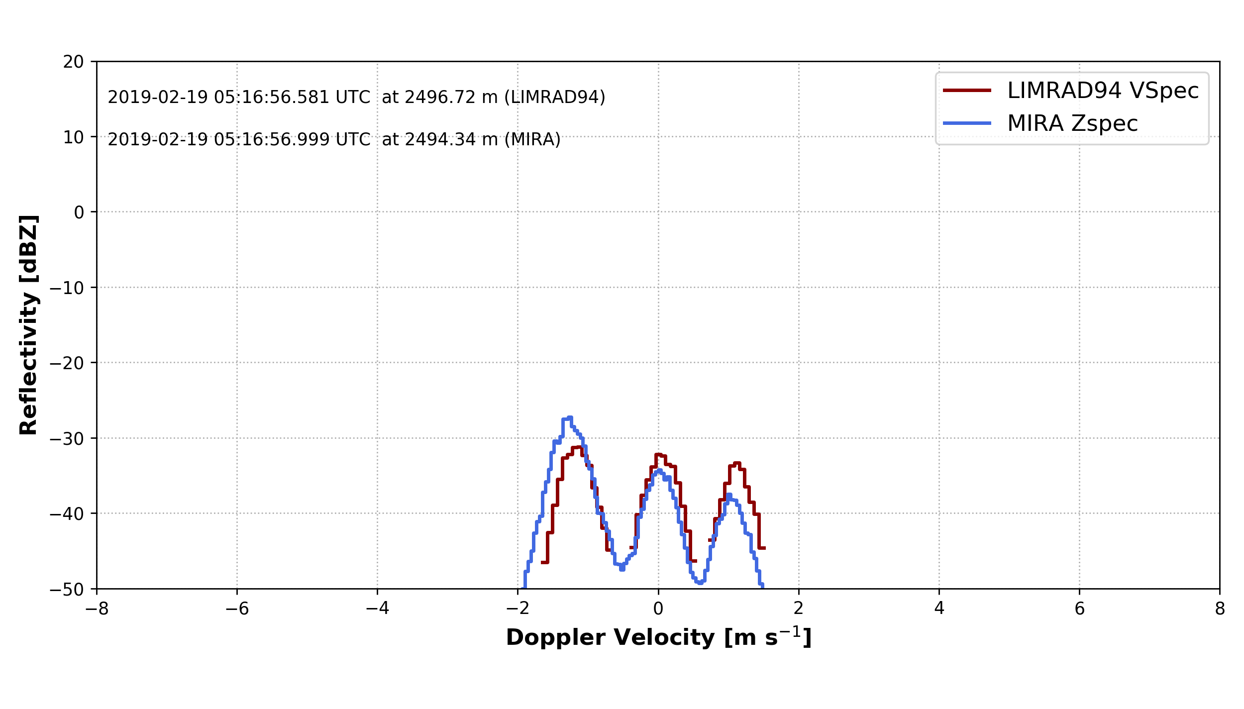
Doppler spectrum

begin_dt = datetime.datetime(2019, 2, 19, 5, 16, 56)
MIRA_Zspec = larda.read("MIRA", "Zspec", [begin_dt], [2490])
LIMRAD94_Zspec = larda.read("LIMRAD94", "VSpec", [begin_dt], [2490])
h.pprint(MIRA_Zspec)
fig, ax = pyLARDA.Transformations.plot_spectra(LIMRAD94_Zspec, MIRA_Zspec, z_converter='lin2z')
fig.savefig('single_spec.png')

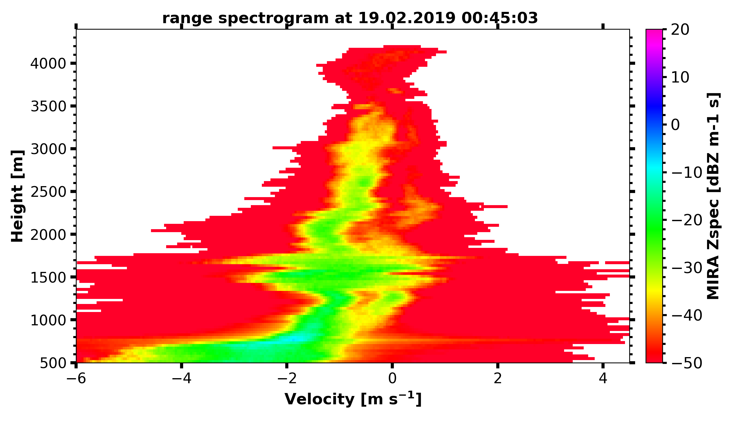
Spectrograms

print('reading in MIRA spectra...')
interesting_time = datetime.datetime(2019, 2, 19, 0, 45, 0)
MIRA_Zspec_h = larda.read("MIRA", "Zspec", [interesting_time], [500, 4400])
print('plotting MIRA spectra...')
fig, ax = pyLARDA.Transformations.plot_spectrogram(MIRA_Zspec_h, z_converter='lin2z', v_lims=[-6, 4.5])
fig.savefig('MIRA_range_spectrogram.png')

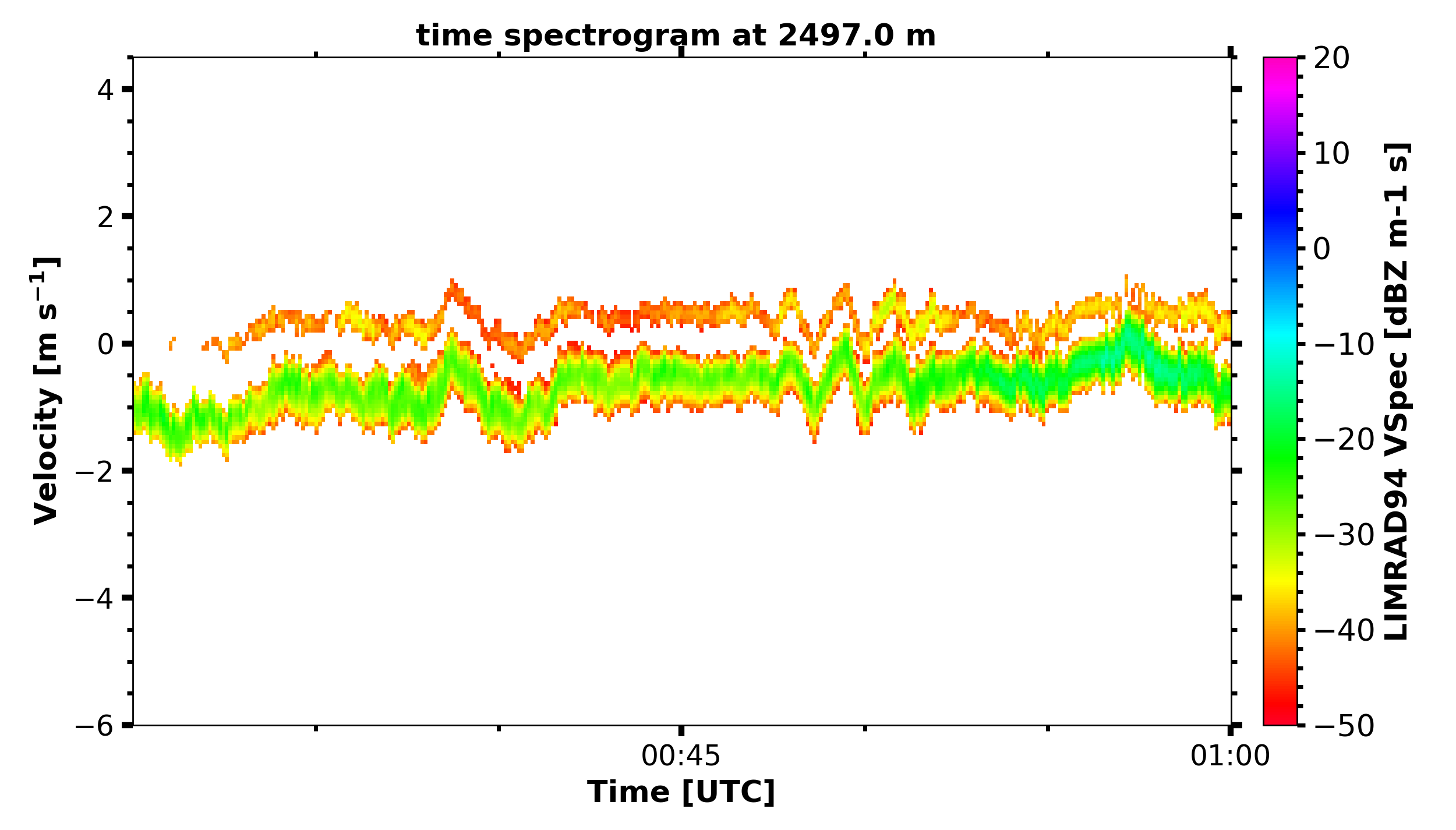
print('reading in LIMRAD spectra...')
begin_dt = datetime.datetime(2019, 2, 19, 0, 30, 0)
end_dt = datetime.datetime(2019, 2, 19, 1, 0, 0)
LIMRAD_Zspec_t = larda.read("LIMRAD94", "VSpec", [begin_dt, end_dt], [2500])
print('plotting LIMRAD spectra...')
fig, ax = pyLARDA.Transformations.plot_spectrogram(LIMRAD_Zspec_t, z_converter='lin2z', v_lims=[-6, 4.5])
fig.savefig('LIMRAD_time_spectrogram.png')

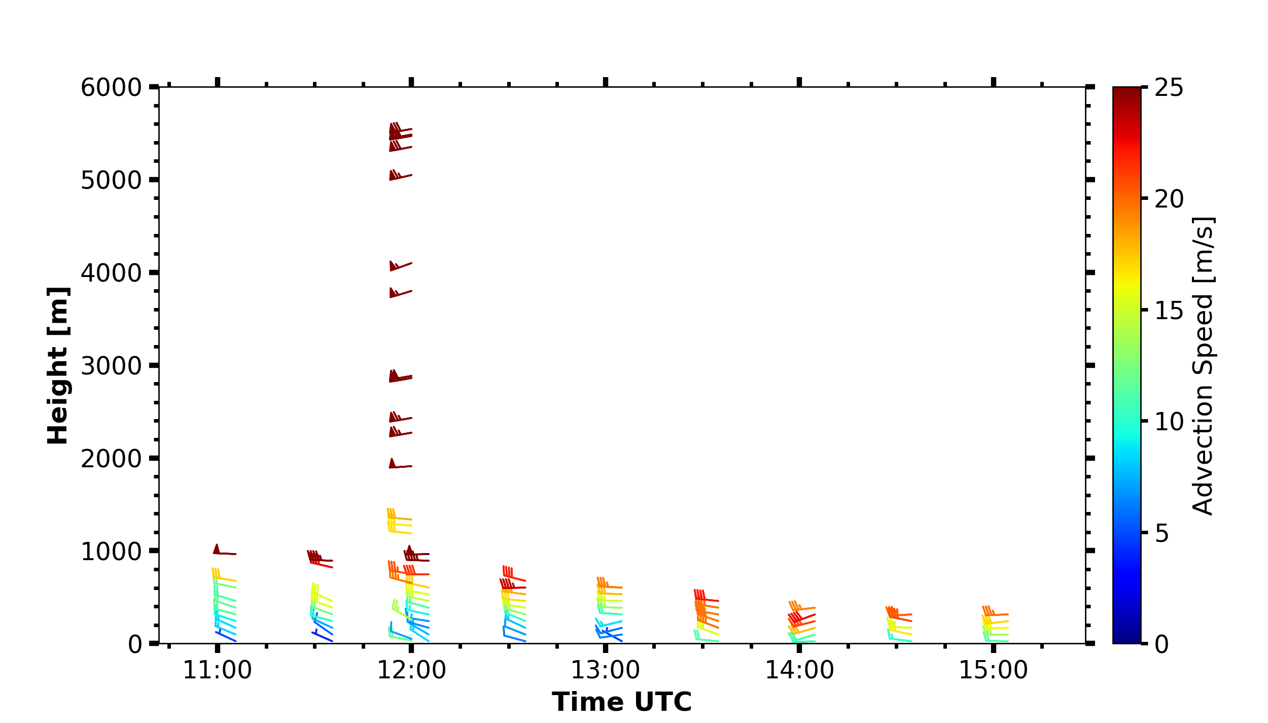
Wind barbs

import pyLARDA.wyoming as uwyo
begin_dt = datetime.datetime(2018, 12, 21, 11, 1, 0)
end_dt = datetime.datetime(2018, 12, 21, 14, 59, 0)

date_sounding = datetime.datetime(2018, 12, 21, 12)
# download the sounding from the uwyo page
wind_sounding = uwyo.get_sounding(date_sounding, 'SCCI')
# load the Doppler lidar u and v components
u_wind_shaun = larda.read( "SHAUN", "u_vel", [begin_dt, end_dt], [0, 'max'])
v_wind_shaun = larda.read( "SHAUN", "v_vel", [begin_dt, end_dt], [0, 'max'])

fig, ax = pyLARDA.Transformations.plot_barbs_timeheight(
    u_wind_shaun, v_wind_shaun, wind_sounding, range_interval=[0, 6000])
fig.savefig('horizontal_wind_barbs.png')

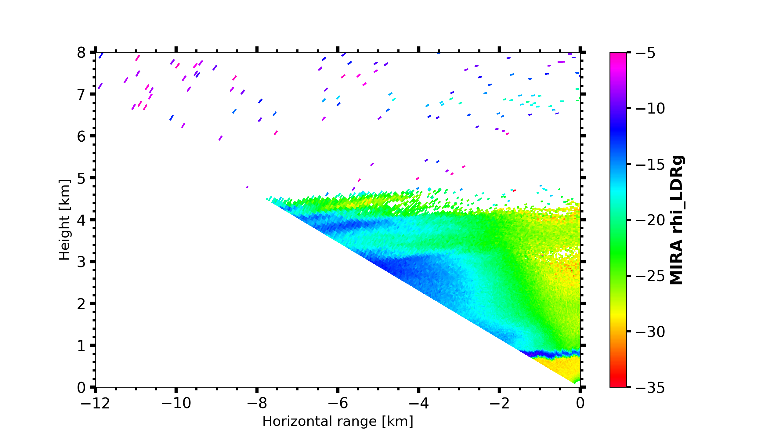
MIRA Scans

dt = datetime.datetime(2019, 4, 18, 21, 30, 0)

MIRA_rhi_SLDR = larda.read("MIRA", "rhi_LDRg", [dt], [0, 'max'])
MIRA_rhi_elv = larda.read("MIRA", "rhi_elv", [dt])

fig, ax = pyLARDA.Transformations.plot_rhi(MIRA_rhi_SLDR,
            MIRA_rhi_elv, z_converter='lin2z')
fig.savefig('MIRA_rhi_scan_SLDR.png')

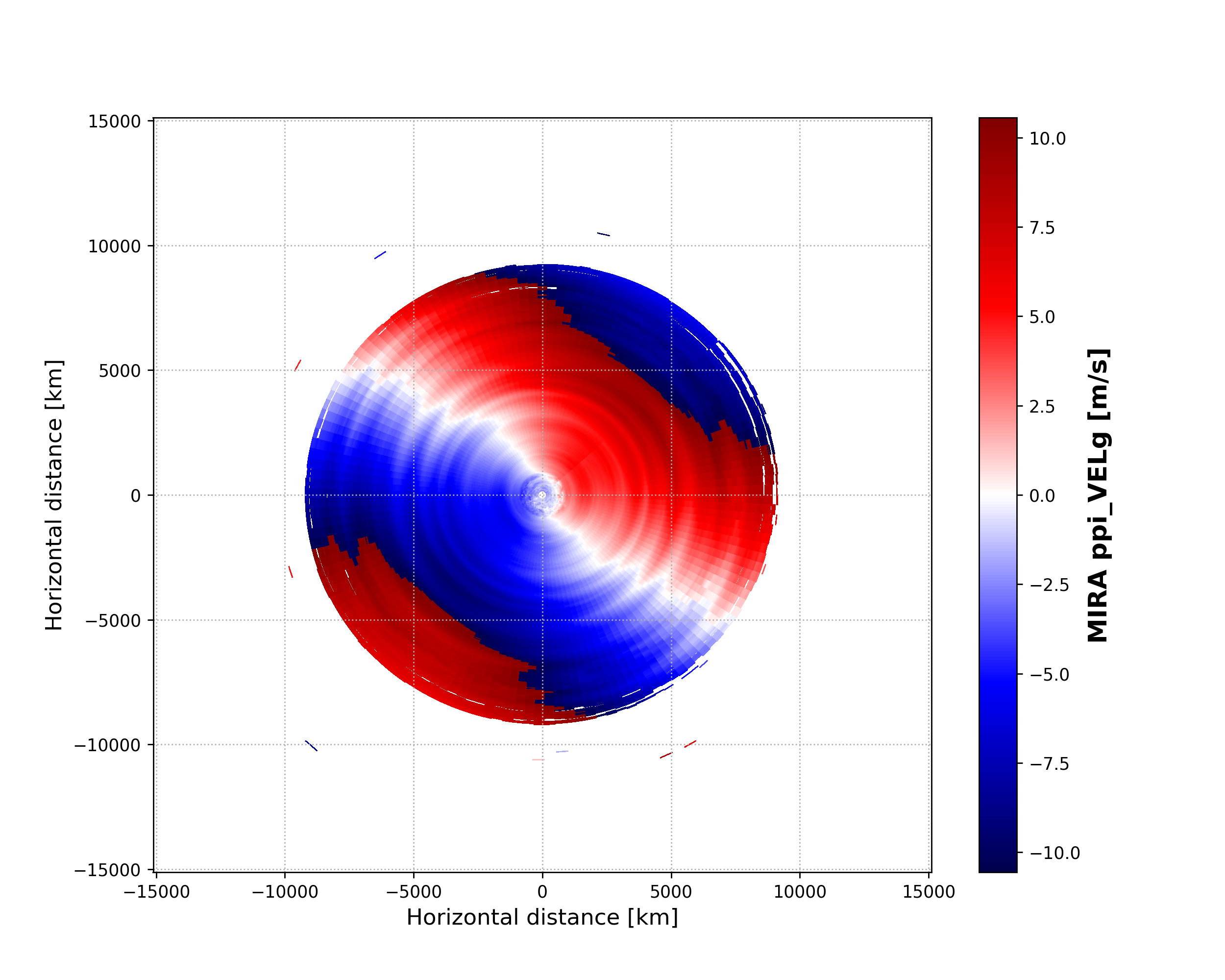
dt = datetime.datetime(2019, 4, 18, 23, 30, 0)

MIRA_ppi_azi = larda.read("MIRA", "ppi_azi", [dt])
MIRA_ppi_vel = larda.read("MIRA", "ppi_VELg", [dt], [0, 'max'])

fig, ax = pyLARDA.Transformations.plot_ppi(MIRA_ppi_vel, MIRA_ppi_azi, cmap='seismic')
fig.savefig('MIRA_ppi_scan_vel.png')

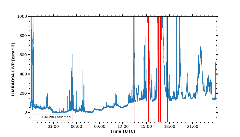
select_closest

Also see for pyLARDA.Transformations.slice_container().

import matplotlib

begin_dt = datetime.datetime(2020, 2, 16, 0, 0, 5)
end_dt = datetime.datetime(2020, 2, 16, 23, 59, 55)

radar_lwp = larda.read("LIMRAD94", "LWP", [begin_dt, end_dt])
hatpro_flag = larda.read("HATPRO", "flag", [begin_dt, end_dt])
# check for HATPRO quality flags
rainflag = hatpro_flag['var'] == 8  # rain flag
if any(rainflag):
    # do not interpolate flags but rather chose closest points to radar time steps
    hatpro_flag_ip = pyLARDA.Transformations.select_closest(hatpro_flag, radar_lwp['ts'])
    rainflag_ip = hatpro_flag_ip['var'] == 8  # create rain flag with radar time
    # get position of flags for vertical lines in plot
    vlines = [h.ts_to_dt(t) for t in hatpro_flag_ip['ts'][rainflag_ip]]
else:
    vlines = []

fig, ax = pyLARDA.Transformations.plot_timeseries(radar_lwp)
if len(vlines) > 0:
    for x in matplotlib.dates.date2num(vlines[:-1]):
        ax.axvline(x, alpha=0.1, color='red')
    # add the last line with label to add to legend
    vline = ax.axvline(vlines[-1], alpha=0.5, color='red', label='HATPRO rain flag')
ax.legend()
fig.savefig("radar-lwp_hatpro-rainflag.png")

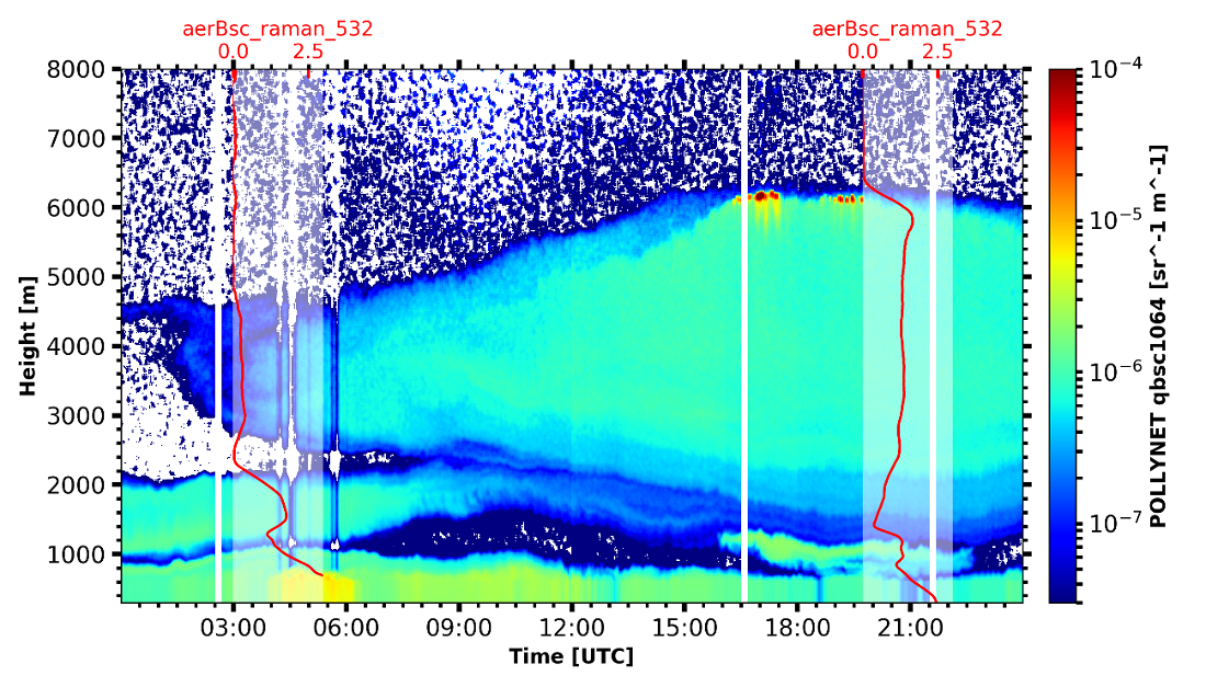
Backscatter with overlay

begin_dt=datetime.datetime(2017,9,14,0,0)
end_dt=datetime.datetime(2017,9,14,23,59)

pollynet_qbsc1064 = larda.read("POLLYNET","qbsc1064",[begin_dt,end_dt],[0,8000])
times = larda.read("POLLYNETprofiles","end_time",[begin_dt, end_dt])

dt = datetime.datetime(2017, 9, 14, 20, 0)
bsc_532 = larda.read("POLLYNETprofiles","aerBsc_raman_532",[dt],[0,8000])

dt = datetime.datetime(2017, 9, 14, 3, 30)
bsc_532_early = larda.read("POLLYNETprofiles","aerBsc_raman_532",[dt],[0,8000])

def add_profile_inset(fig, ax, bsc_532, rel_xloc):
    # print(h.ts_to_dt(bsc_532['ts']))
    # print(h.ts_to_dt(pollynet_qbsc1064['ts'][-1])-h.ts_to_dt(pollynet_qbsc1064['ts'][0]))

    inset_width = 0.1
    print('calculated inset x position ', rel_xloc)

    # add an inset plot with the 'proper profile'
    # These are in unitless percentages of the figure size. (0,0 is bottom left)
    from mpl_toolkits.axes_grid1.inset_locator import inset_axes
    axins = inset_axes(ax, width="100%", height="100%",
                    bbox_to_anchor=(rel_xloc, 0.00, inset_width, 1),
                    bbox_transform=ax.transAxes, borderpad=0)
    # actually plot the profile
    axins.plot(bsc_532['var'][0,:]*1e6, bsc_532['rg'],
            color='red', label='532')
    # make a faint background
    axins.patch.set_facecolor('white')
    axins.patch.set_alpha(0.5)
    # set the height interval of the inset similar to the colorplot
    axins.set_ylim(range_interval)
    axins.set_xlim(0,3)
    #axins.axes.get_yaxis().set_visible(False)
    #spines are the borders of the inset plot
    axins.spines['left'].set_visible(False)
    axins.spines['right'].set_visible(False)
    # disable the tick marks of the inset plot
    axins.tick_params(axis='both', left=False, top=True, right=False, bottom=False,
                    labelleft=False, labeltop=True, labelright=False, labelbottom=False)
    # label the inset axis on top
    axins.set_xlabel(bsc_532['name'], color='red', fontsize=12)
    axins.xaxis.set_label_position('top')
    axins.tick_params(axis='both', which='major', labelsize=12,
                    direction='in', color='r', labelcolor='r', width=2, length=5.5)

    return fig, ax, axins


# make the colorplot with the usual Transformations.plot_timeheight(...)
range_interval = [300, 8000]
fig, ax = pyLARDA.Transformations.plot_timeheight(
    pollynet_qbsc1064, range_interval=range_interval, var_converter='log')

# add first profile
rel_xloc = (bsc_532['ts'][0]-pollynet_qbsc1064['ts'][0])/ \
                (pollynet_qbsc1064['ts'][-1]-pollynet_qbsc1064['ts'][0])
fig, ax, axins = add_profile_inset(fig, ax, bsc_532, rel_xloc)

# and the second one
rel_xloc = (bsc_532_early['ts'][0]-pollynet_qbsc1064['ts'][0])/ \
                (pollynet_qbsc1064['ts'][-1]-pollynet_qbsc1064['ts'][0])
fig, ax, axins = add_profile_inset(fig, ax, bsc_532_early, rel_xloc)

fig.subplots_adjust(top=0.90)
fig.savefig('POLLYNET_quasi_bsc_with_inset.png', dpi = 250)

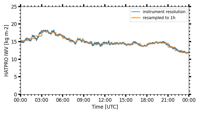
xarray resample and plot

Also see for pyLARDA.Transformations.container2DataArray() and pyLARDA.Transformations.plot_timeseries2().

larda_rsd2.connect('lacros_cycare')
begin_dt = datetime.datetime(2018, 1, 15, 0, 0)
end_dt = datetime.datetime(2018, 1, 16, 0, 0)

iwv = larda_rsd2.read('HATPRO', 'IWV', [begin_dt, end_dt])

iwv_xr = pyLARDA.Transformations.container2DataArray(iwv)

iwv_resampled = iwv_xr.resample(time="1H", keep_attrs=True).mean(keep_attrs=True)

fig, ax = pyLARDA.Transformations.plot_timeseries2(
    iwv, figsize=[7,4], label='instrument resolution')
fig, ax = pyLARDA.Transformations.plot_timeseries2(
    iwv_resampled, tdel_jumps=4000, step='post',
    linewidth=2, label='resampled to 1h',
    fig=fig, ax=ax)
ax.legend()

fig.savefig("hatpro_iwv_resampled.png")